Animating an isochrone map

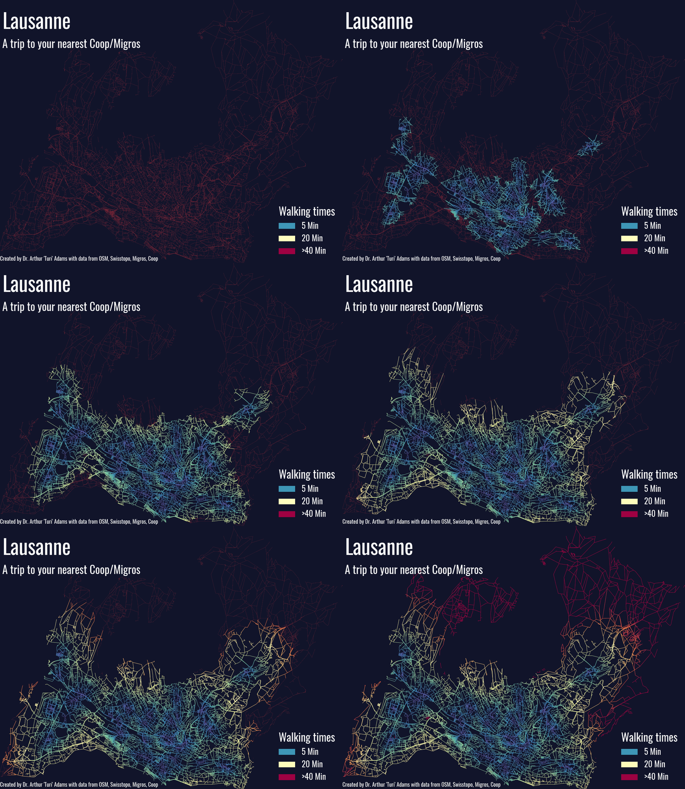
In the last post about producing isochrone walking maps we learnt how to produce an isochrone map, here we will learn how to easily animate it using Matplotlib’s FuncAnimation.

How to use FuncAnimation

Here is an example of FuncAnimation:

animation = FuncAnimation(fig, 
                          animate_map, 
                          frames=times, 
                          init_func=init_map, 
                          interval=100, 
                          repeat = True)
animation.save("YourFileName.gif")
plt.show()

First, we define a figure fig where our animation will take place, then we set a function animate_map that updates the map on each frame. The frames are set to a variable times, which is just a list from 0 – 40, which will be passed to the animate_map function. Init_func is the function that sets up the first frame of the animation before animate_map is called. The interval refers to the milliseconds between each frame – in this case 100 ms a frame – and we set the animation to repeat.

Then we must save the animation to get it to run, and we use plt.show() to show the animation.

Now let’s go through the functions and variables starting with times.

times = list(np.arange(40))
times.extend([40,40,40,40,40,40,40])

Times is list of numbers from 0 to 40, that is concatenated with a list of the number 40 seven times. By adding the extra 40’s, we are telling the frames to continue showing the last frame (that where the times = 40 minutes) for an additional 700 ms (100 ms a frame) before repeating. This allows the figure to “breath” and settle with the viewer before repeating.

Now here is our initialization function:

def init_map():
    ax.set_xlim(minx, maxx)
    ax.set_ylim(miny, maxy)
    ax.set_axis_off()
    lines_df.plot(ax=ax, 
                  column='Line_value', 
                  color='#bb3443', 
                  alpha=0.3, 
                  linewidth=0.6)
    lacLeman.plot(ax=ax, facecolor="#032a4b")
    ax.annotate("Lausanne", 
               (minx+100,maxy-1200), 
               color="White", 
               fontsize=25, 
               font=font, 
               weight='bold' )
    ax.annotate("A walk to your nearest Coop/Migros", 
               (minx+100,maxy-2000), 
               color="White", 
               fontsize=12, 
               font=font, 
               weight='bold' )
    ax.legend(handles=legend_elements,
             title='Walking times',
             alignment='left',
             title_fontproperties=font, 
             loc='lower right', 
             framealpha=0, 
             labelcolor="White",
             prop=font,
             fontsize='40')
    ax.get_legend().get_title().set_color('White')
    ax.get_legend().get_title().set_fontsize('24')
    plt.legend

The two dataframes are lines_df, which contains LineStrings of our road network, and lacLeman, which is a shapefile of the Lac Leman.

There is nothing of note here, which is different from what we did in step 8 of How to make an isochrone walking map.

Let’s move on to the animate_map() function:

def animate_map(time):
    ax.clear()
    lines_df.plot(ax=ax, 
                  column='Line_value', 
                  edgecolor='#bb3443', 
                  alpha=0.3, 
                  linewidth=0.6)
    ax.set_xlim(minx, maxx)
    ax.set_ylim(miny, maxy)
    ax.set_axis_off()
    lines_df.loc[lines_df['Line_value'] <= time].plot(ax=ax,   
                column='Line_value', 
                cmap=cmap, 
                linewidth=0.6, 
                vmin=0, 
                vmax=40)
    lacLeman.plot(ax=ax, facecolor="#032a4b")
    ax.annotate("Lausanne", 
                (minx+100,maxy-1200), 
                color="White", 
                fontsize=45, 
                font=font, 
                weight='bold' )
    ax.annotate("A trip to your nearest Coop/Migros", 
                (minx+100,maxy-2000), 
                color="White", 
                fontsize=24, 
                font=font, 
                weight='bold' )

    ax.legend(handles=legend_elements,
             title='Walking times',
             alignment='left',
             title_fontproperties=font, 
             loc='lower right', 
             framealpha=0,
             labelcolor="White",
             prop=font,
             fontsize=18)
    ax.get_legend().get_title().set_color('White')
    ax.get_legend().get_title().set_fontsize('24')
    plt.legend

The differences between animate_map and init_map are that we must clear the axes object after each frame with ax.clear(), because otherwise we would be overwriting the axes object with the next plot. For example imagine you annotate a title that shows the frame number of each frame, if you don’t clear it, each number would be plotted overtop of the last one as each frame is rendered creating a jumble of mashed numbers. So clear your axes.

The only other thing to note is that now lines_df is filtered for only values that are less than or equal to the time. The frames go as follows:

Frame 1: show only the basemap (time = 0).
Frame 2: show time <= 1 minute.
Frame 3: show time <= 2 minutes.
etc

Put that all together and you get something like this!

How to use FuncAnimation

Leave a Reply Cancel reply