I started this project thinking, what would it look like, if we were to start in the geographic center of Switzerland and drive out to every single municipality?

In other countries these maps show radiating roads from a country’s center , but here in Switzerland the Alps are a formidable barrier between the South and North and municipalities often have unique and ancient shapes.

So in this tutorial we will find the most optimal driven route from the center of Switzerland to each and every reachable Swiss municipality.

1. Initialization

We have lot’s of ground to cover here.

Let’s begin with our standard imports, of which Pandana is the only unique library that will be used for the network analysis:

import geopandas
import pandana
import pathlib
import pandas as pd
import numpy as np
from shapely import LineString
from pandana.loaders import osm
from matplotlib import pyplot as plt

Next we will import our layers beginning with the road network of Switzerland. This network can be obtained using the Pandana loader osm.pdna_network_from_bbox(), which takes the coordinates of the bounding box and the type of network.

Switzerland’s road network is obtained as follows:

#Took me about 6 minutes to obtain the network
network = osm.pdna_network_from_bbox(45.818, 5.9559,47.8084,10.4921, network_type='drive')
lcn = network.low_connectivity_nodes(10000,10,imp_name='distance')
network.save_hdf5(DATA_DIRECTORY /'driving_network_Switzerland.h5', rm_nodes=lcn) 

Note: we specify “drive” to obtain the road network instead of the pedestrian or “walking” network, and the boundary boxes are in WGS 84 decimal degrees. After we obtain the network, we create another parameter called lcn, which defines the removal of low connectivity nodes – or those isolated here by over 10000 meters or 10 connections. By default the imp_name (impendence) is equal to distance for Pandana objects.

Finally we save it as a HDF5 file and pass lcn to the rm_nodes parameter. If you are not interested in removing low connectivity nodes, feel free to omit creating the lcn object.

Great! With that in order let’s define our paths and target layers beginning with our highway nodes:

switzerland_roads_network = pandana.network.Network.from_hdf5(DATA_DIRECTORY / 'driving_network_Switzerland.h5')
switzerland_road_network_nodes = geopandas.GeoDataFrame(switzerland_road_network.nodes_df,                                 geometry=geopandas.points_from_xy(switzerland_road_network.nodes_df.x,                                                                           switzerland_road_network.nodes_df.y),                                                                crs='EPSG:2056')

Using the .h5 file we made, let’s load it as a Pandana network, then use its nodes, which are contained as a dataframe from network_name.nodes_df, to create a GeoDataFrame. Finally we reset the index, so that we can access the id of the nodes as a column in the GeoDataFrame.

Right now, switzerland_road_network_nodes contains all of the nodes within the defined bounding box, meaning it also contains nodes from Germany, Italy, France and Liechtenstein. Therefore we need to remove those nodes, and keep only the ones in Switzerland.

#Get shape of Switzerland and make it into a single polygon
switzerland = geopandas.read_file(DATA_DIRECTORY / "swissBOUNDARIES3D_1_5_LV95_LN02.gpkg", layer="tlm_hoheitsgebiet")
switzerland = switzerland.loc[switzerland["icc"]=="CH"]
switzerland_shape = switzerland.dissolve()
switzerland_shape.rename(columns={0:"geometry"}, inplace=True)
switzerland_road_network_nodes.reset_index(inplace=True)
nodes_in_Switzerland = switzerland_road_network_nodes.overlay(switzerland_shape, how='intersection')

Here we load the swissBOUNDARIES3D geopackage from swisstopo, and we extract the tlm_hoheitsgebiet layer to get a shapefile of Switzerland. Then we filter the shapefile with icc=CH to only select the boundaries within Switzerland, the shape is dissolved into one polygon, and we finally rename the geometry column.

Then we find the intersection between the nodes and the Switzerland polygon to get all the nodes within Switzerland.

Finally we import the waterways layer tlm_bb_bodenbedeckung for the map from SwissTLM3D:

water = geopandas.read_file(DATA_DIRECTORY_RASTER / 'SWISSTLM3D_2024_LV95_LN02.gpkg', layer='tlm_bb_bodenbedeckung') 

That was a lot of work just to initialize the network, but now we are basically ready to begin … after a little bit more cleanup.

2. A bit more data clean up

Before getting into the analysis, we need to clean up our edges. Right now, our switzerland_roads_network contains all the edges within the bounding box, including those outside of Switzerland.

To remove those edges we do the following:

edges_in_Switzerland = switzerland_roads_network.edges_df[switzerland_roads_network.edges_df['from'].isin(nodes_in_Switzerland['id']) & switzerland_roads_network.edges_df['to'].isin(nodes_in_Switzerland['id'])]

Just like switzerland_roads_network had an nodes_df attribute, it also has a edges_df attribute that can be filtered to only include nodes within Switzerland.

Next we create a new network with only nodes and edges within Switzerland:

#Important to set the index back for later on
nodes_in_Switzerland.set_index('id', inplace= True)
switzerland_road_network = pandana.Network(nodes_in_Switzerland['x'], nodes_in_Switzerland['y'], edges_in_Switzerland['from'], edges_in_Switzerland['to'], edges_in_Switzerland[['distance']])

In Pandana dataframes, distance is the default name of the impedance column.

Now our switzerland_road_network truly only represents Switzerland.

3. Defining the center and pre-function variables

The geographical center of Switzerland is a little place called Älggi-Alp in the canton of Obwalden. To obtain the nearest node to the coordinates of Älggi-Alp, we run:

center_switzerland_node_id = switzerland_road_network.get_node_ids([8.226667], [46.801111]).iat[0]
# 3622400917

Here it’s important that the order of your input is longitude, then latitude, or East then North, and that it matches the CRS of your network, which in this case is WGS 84.

Let’s also create a results DataFrame and get the ID’s of all the target municipalities, which are designated as bfs_nummer:

results = pd.DataFrame(columns=['id','x','y','geometry','bfs_nummer'])
bfs_nummern = switzerland.bfs_nummer.unique()

4. Finding the optimal route to each municipality

This will be a big code block, but just follow the comments and you’ll do fine. Essentially, we are looping through each municipality bfs number and:

1. Create a shape of the municipality
2. Find all nodes within the municipality
3. Check to make sure the muncipality is not 1406, which is the municipality of Sachseln, or the home to Älggi-Alp – so the shortest distance would be 0. We also check to make sure there are nodes in the target municipality, because some of the bfs numbers refer to lakes.
4. We create a dataframe that is populated with two columns, 1 the origin node id and 2 the nodes in the target municipality.
5. We get the shortest path between each node couple.
6. We find the minimum distance of all the node couples, and therefore the shortest distance to the municipality.
7. We collect the nodes along that path.
8. Place those nodes within a DataFrame along with the bfs number.
9. Then we make Linestrings between the edges.
10. Finally we concatenate the results DataFrame with the path to the municipality.

And all that looks like this:

for num in bfs_nummern:
    print(num, ' Beginning')
    target_muni = switzerland.loc[switzerland['bfs_nummer'] == num]
    muni_unified = target_muni.dissolve()
    muni_unified.rename(columns={0:"geometry"}, inplace=True)
    muni_unified.set_geometry("geometry", inplace=True)

    nodes_in_target_muni = nodes_in_Switzerland.overlay(target_muni, how='intersection')
    if not nodes_in_target_muni.empty and num != 1406:
        origin_destination_nodes = pd.DataFrame({'destination':nodes_in_target_muni['id'].values})
        origin_destination_nodes['origin'] = center_switzerland_node_id
        
        #Get shortest distances
        origin_destination_nodes['distances'] = switzerland_road_network.shortest_path_lengths(origin_destination_nodes.origin.values, origin_destination_nodes.destination.values, 'distance')
        
        node_id_shortest_path_to_muni = origin_destination_nodes.loc[origin_destination_nodes['distances'] == origin_destination_nodes['distances'].min()]
        
        shortest_path_to_muni_nodes = switzerland_road_network.shortest_path(center_switzerland_node_id, node_id_shortest_path_to_muni['destination'].iat[0], 'distance')
        
        nodes_in_target_muni_path = nodes_in_Switzerland.loc[nodes_in_Switzerland['id'].isin(shortest_path_to_muni_nodes)]
        nodes_in_target_muni_path = nodes_in_target_muni_path[['id','x','y','geometry','bfs_nummer']]
        nodes_in_target_muni_path = nodes_in_target_muni_path.set_index('id').reindex(shortest_path_to_muni_nodes).reset_index()
        nodes_in_target_muni_path.loc[:,'bfs_nummer'] = num

        #Make Linestrings
        data_offset = nodes_in_target_muni_path.copy().iloc[1:]
        data_offset.reset_index(inplace=True)
        data_offset.rename(columns={'geometry': 'to_geometry'}, inplace=True)
        combined = pd.concat([nodes_in_target_muni_path, data_offset['to_geometry']],axis=1)
        combined = combined.copy().iloc[:-1]
        combined['geometry_path'] = combined.apply(lambda row: LineString([row['geometry'],row['to_geometry']]), axis =1)

        results = pd.concat([results,combined]).copy()

On my medium spec computer this takes about 33 minutes to run, so once it’s done I save it as a geopackage.

map = geopandas.GeoDataFrame(results, geometry='geometry_path',crs="EPSG:2056")
export = map.drop(['geometry','to_geometry'], axis=1)
export.to_file(DATA_DIRECTORY / 'pathsToAllGemeinden.gpkg')

5. Plotting

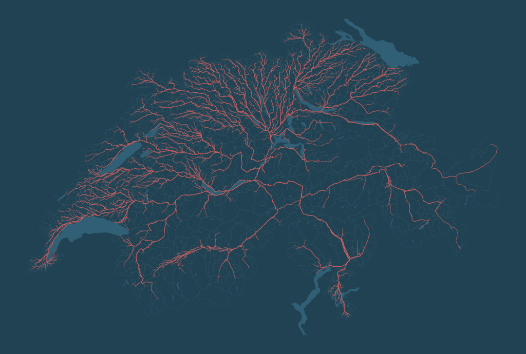
Unlike the last few tutorials, plotting the map is quite simple:

#Filter the water file to only show still water
water_shape = water.loc[water['objektart'] == 'Stehende Gewaesser']

fig, ax = plt.subplots(figsize=(25,25))
fig.set_facecolor("#214252")
switzerland.plot(ax=ax, column='bfs_nummer', facecolor='None', edgecolor='#4e6d7d', linewidth=0.2, antialiased=True)
export.plot(ax=ax, color='#ce6262',linewidth=1.5)
water_shape.plot(ax=ax, edgecolor=None, facecolor='#305F76')
ax.set_axis_off()

And there you have it:

6. Wrapping up

As is typical, most of the work was spent cleaning up our data instead of doing the analysis. I would also argue that there are more efficient ways of getting the shortest distance and in fact Pandana has a method shortest_paths, which is a vectorized version of the shortest_path method used here and should be much faster. Since this was a one time project, I didn’t bother adapting the code for it but it’s definitely something you could look into.

Find more information about the Pandana API .